Excel Tips for Evergreen Reports

Microsoft Excel 2010

Concepts

Evergreen reports are available as spreadsheets in Excel or CSV format. This allows you to manipulate the data, and customize the reports to best meet your needs and interests. This page outlines some key Excel tips for working with Evergreen reports.

These instructions and images use Excel 2010.

Multi-worksheet reports

Many Evergreen reports (a single Excel workbook) are composed of multiple worksheets. Individual sheets are indicated at the bottom of the Excel window with tabs. Each worksheet has its own name (default: Sheet 1, Sheet 2 or custom: Local Demand, System Demand) which appears in the tab. The active worksheet/tab is white, the others are grey. Click on a tab to open that worksheet. When your workbook has a large number of worksheets they may not all display; use the arrow icons to the left of the worksheet tabs to navigate to the first, previous, next, or last worksheet.

Add a new worksheet

At the end of the row of worksheet tabs in a placeholder icon, click on this icon to add a new sheet. It will be named Sheet2.

Rename a worksheet

1. Right Click on the tab to change
2. Select Rename
3. Type the new tab name
4. Save the worksheet

Re-order worksheets

To re-order worksheets, click-an-hold on the tab until a small black arrow and page icon appear. Drag the mouse so that the down arrow is in the new worksheet position and release.

Select cells

Select a single cell

Click in the specific cell. Editing, formatting, or copy/pasting options will apply only to the selected cell.

Select all cells

Whenever you need to select all cells (such as to apply formatting) in a worksheet, click in the upper left most square, where the row headers and column headers intersect. The entire worksheet will be highlighted.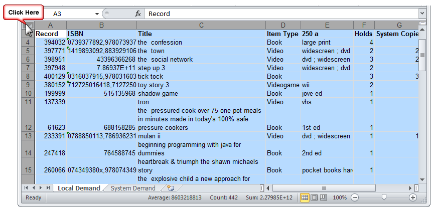

Select an entire column or row

Whenever you need to select all cells in column or row:

1. Click on the column or row header. The entire column or row will be highlighted.

To select contiguous columns or rows:

1. Click on the first header
2. Drag the cursor over the desired headers to select

To select non-contiguous columns/rows:

1. Click on the first header
2. Press and hold the Ctrl key and click on desired headers to select

Select a column:

Select a row:

Display cell data in the formula bar

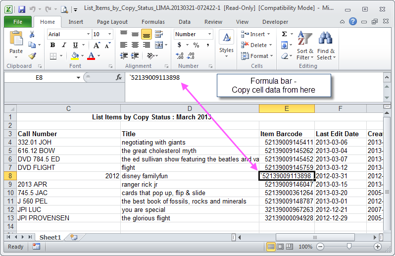
The formula bar displays the formula underneath the data that displays in the cell itself. This will allow you to edit the formula - for example, if the wrong cells were selected for a sum.

It will also show you the original data from an Evergreen report when the Excel program has changed the data according to some formula - for example, when the data from evergreen is a barcode, when a barcode contains leading spaces, and other issues.

Turn on the formula bar

Generally, the formula bar displays by default, in a row beneath the ribbon and above the table. If it does not, enable this feature:

1. Click View
2. In the View ribbon, click Show
3. Check Formula Bar

View data in the formula bar

1. Select the cell
2. The data displays in the formula bar
3. Highlight the data to copy and paste into ItemStatus

Change barcode / ISBN format

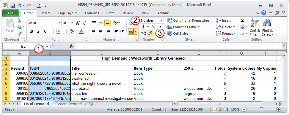
When most reports containing barcode and ISBN cells are opened in Excel, the barcode numbers and ISBNs are expressed in scientific notation. To change these to the actual values you need to change the data-type for the cells.

1. Highlight the entire column(s) to change
2. In the Home menu tab, Number area
3. Change the Number Format to Number; the barcodes and/or ISBNs will display as: 9780385528047.00
4. Click the Decrease Decimal button twice to remove the decimal and the zeroes

Text to Columns

Often when pasting information into Excel (such as when using CopyListCsvToClipboard), all data is pasted into the A1 cell. In this situation, use the Text to Columns function to sort data into the appropriate columns.

1. Copy data from the source application
2. Open a blank Excel worksheet
3. Paste the data into the blank worksheet
4. Select all of column A
5. In the Data menu, Data Tools area
6. Click Text to Columns
7. The Convert Text to Columns Wizard opens, this is a 3 step process
8. Step 1 - click delimited, click Next
9. Step 2 - select delimiters, click Next
   • A delimiter is a character that indicates what pieces of information go together, as in a single cell; the delimiter is different based on the source data. Evergreen CSV data is comma delimited
   • The data preview will insert lines where the data will split into columns; if this does not look correct, change the delimiter
10. Step 3 - Click Finish
11. All data displays in columns, with no commas or quotation marks

Auto-fit column width and row height

Size all column widths and row heights to fit the cell contents:

1. Select all cells
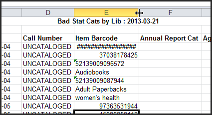
2. Place your cursor on the border between two column headers, until the cursor looks like a vertical line crossed by a horizontal arrow, then double click; all columns expand or contract to the width of the longest content string
3. Place your cursor on the border between two row headers, double click; all rows expand or contract to the height of the tallest content string

Size a single column or row to the cell contents:

1. For the column to adjust, place your cursor on the right side border of the column header, double click; the column expands or contracts to the width of the longest content string
2. For the row to adjust, place your cursor on the lower border of the row header, double click; the row expands or contracts to the width of the tallest content string

Manually fit column width and row height

Sometimes, typically with Title information, the contents of a cell are too long to autofit the column or row. To manually adjust:

1. Place your cursor on the right border of the column header or lower border of the row header until the cursor looks like a vertical line crossed by a horizontal arrow
2. Click and drag the cell to the appropriate width/height.

Hide / Unhide Columns

When a report is very wide, you can hide columns in order to make sorting the list easier to handle. The columns can be un-hidden to view the data.

1. Click in a column header to select the columns, or click and drag to select multiple columns
2. Right click, in the menu select Hide
3. The columns collapse

To un-hide the columns

1. Place your cursor in the header row over the space indicating the hidden columns
2. Right click
   • A column should not be select, instead you should see the menu and a heavy line between the columns
3. Click Un-Hide
4. The columns display

Wrap Text

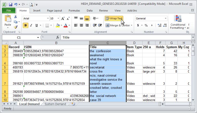
If the contents of a cell are too long to display in a column, but you still wish to see all of the content, use wrap text.

1. Highlight a single cell or the entire column
2. In the Home menu tab, Alignment area, click Wrap Text
3. The row heights will adjust to fit all cell contents, the column wdith will remain the same

Sorting

Custom Sort

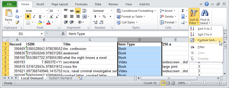
Use for sorting by a single column, or to create a mutiple column, nested sort. This ensures that all rows in a table are kept together when sorted.

1. Click on any data cell in the worksheet
2. In the Home menu tab, Editing area
3. Click Sort & Filter
4. Click Custom Sort
   
5. At the Sort Warning, select Expand the Selection and click Sort
   
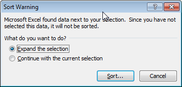
   • This selects all columns in the worksheet; if you have already selected all columns, this warning will not appear
6. Select Sort by values; add levels as needed
   
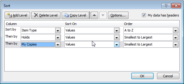
7. Click OK

This method is recommended - all records remain intact, multiple sorting criteria can be selected, and sort options can be set per level

Select data to sort

If your worksheet contains a title row, merged cells, or other content you do not wish to (or cannot) sort you need to select the data

1. Click on a data cell in your worksheet
2. Use the keyboard shortcut: CTRL+Shift+* (this selects the region around the active cell - the data area enclosed by blank rows and blank columns.)

Filtering

When working with a large worksheet you may be interested in only one segment of the data. Use a filter to view and print selected segments of data.

1. Click on a data cell in your worksheet
2. In the Home menu tab, Editing area
3. Click Sort & Filter
4. Click Filter
   
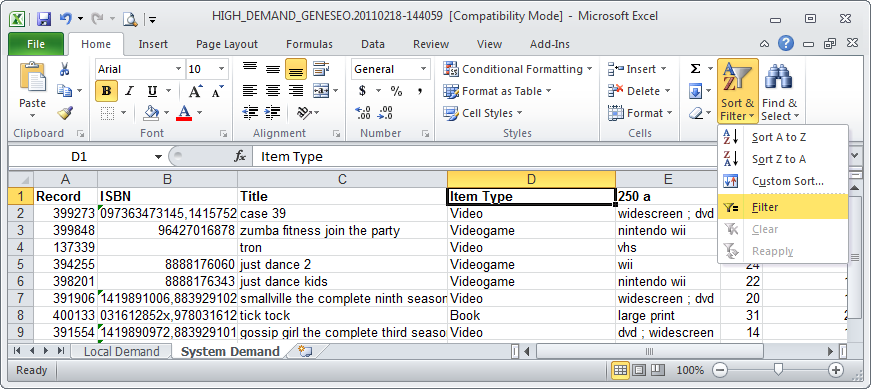
   arrows will be inserted into the column labels
5. Click on the arrow in the column you wish to filter to select your filter options
   
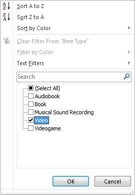
   • Filter by text - the filtered records will only include that word
   • Filter by a selected value - the filtered records will only include that value
6. Click OK
7. Additional columns can be filtered to further refine the data set

Filtered columns are indicated by a funnel icon displays in the column label
The records retain their original row numbers; the records filtered out are hidden.

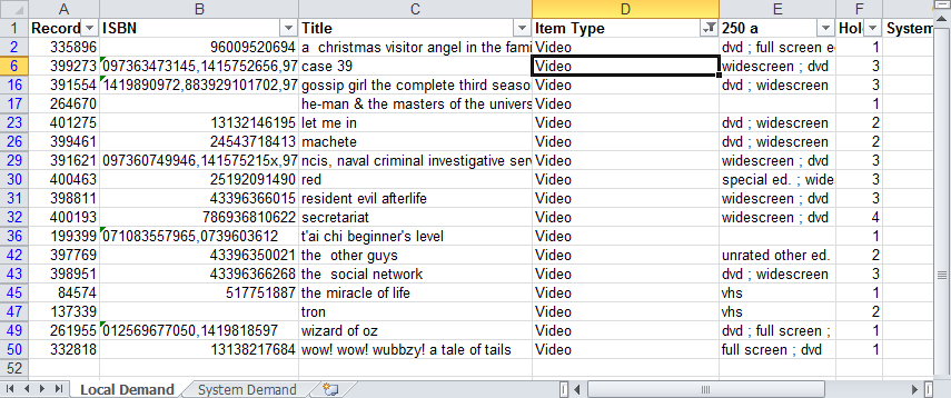
Remove a filter

If you have applied multiple filters, it is recommended that you remove the filters in reverse order

1. Click on the column funnel icon
2. Click Remove filter from "[Column Label]"

Page layout for printing

Select print area

1. Select the range of cells to print
2. In the Page Layout menu tab, Page Setup area, click Print Area
3. Click Set Print Area; the cells are outlined by a dashed line
4. Print the worksheet
5. To remove the print area, click Print Area, click Clear Print Area

If the data is resorted, the same print are will remain

If columns or rows are inserted within the print area they will be included in the print area

Force worksheet to print to specified page width/height

In the Page Layout menu tab, Scale to Fit area you can select the number of pages wide and the number of pages long you wish the worksheet to be. Be default, these are set to "Automatic" which equal 100% scale.

Selecting fewer pages wide or long reduces the scale of the worksheet, and results in smaller font size for the printed result.

For very wide worksheets you may want to use this in conjunction with landscape page orientation, hiding columns, and/or manually resizing columns to minimize wasted space.

Change page orientation

1. In the Page Layout menu tab, Page Setup area
2. Click Orientation
3. Select Portrait or Landscape; new worksheets are by default Portrait

Print gridlines

1. In the Page Layout menu tab, Sheet Options area
2. Under Gridlines, check Print

Print preview and settings

1. Click File
2. Click Print

This opens print preview and provides an opportunity to adjust page setup before printing.

Settings

All changes in settings will display in the preview pane

• Print Active Sheet - the sheet currently active, you can also opt to print the entire workbook (for multi-sheet workbooks)
• Print specific pages - specify page numbers
• Print one-sided - you can also opt to print double-sided, and select the print orientation
• Collation
• Page orientation - use Landscape for wide reports, use in conjunction with the scaling option "Fit all columns on one page"
• Paper size
• Margins - use preset options or enter custom margin widths to change the amount of text that will fit per page
• Scaling - change the relative text size to determine how much of the report fits on the printed page
  • No Scaling - 100% text size
  • Fit sheet on one page - the entire worksheet will print to one page (depending on how big the worksheet is, this could result in very small text)
  • Fit all columns on one page - keeps all columns together, useful in conjunction with Landscape orientation
  • Fit all rows on one page - often similar result as "Fit sheet on one page" option

The Print dialog is a good candidate for adding to the Quick Access Toolbar

Sums and sub-totals

Auto-sum

1. Click in the empty cell at the end of the column or row to sum
2. Click the Formulas menu tab
3. Click AutoSum
4. Click Sum
5. Press Enter

Enter a formula manually

1. Click in a cell where you want the total
2. Type: =SUM(
3. Select the data cells to total, press Enter

Insert Subtotals

Of the PLS reports, this function is most likely to be used with the Reports Monthly New Users

1. Open and save a New Users report
2. Click on a cell in the StatCat Type column
3. Click on the Data menu tab
4. Click on the Subtotal icon
5. In the Subtotal wizard, make sure that:
   • At each change in: = StatCat Type
   • Use function: = Sum
   • Add subtotal to: = New Users is checked
   • Summary below data is checked
6. Click OK
7. Subtotal rows are inserted for Patron Type, Residency, and School Code

Download PDF instructions

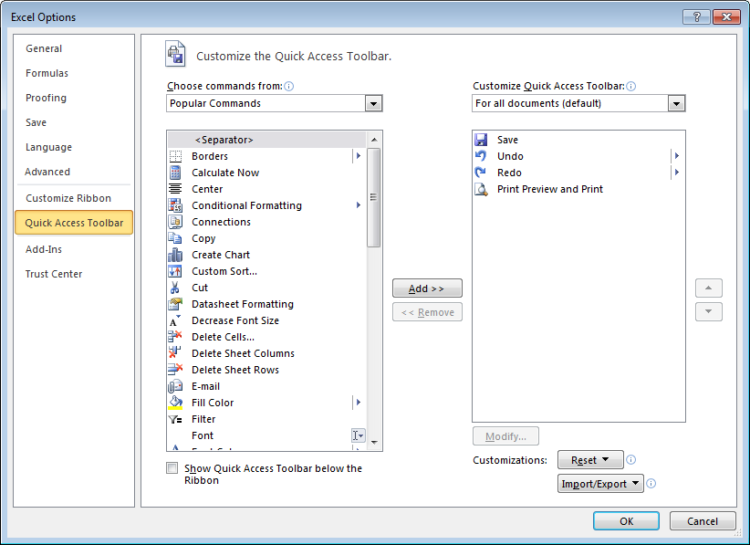
Add commands to the Quick Access Toolbar

If you use specific commands frequently, you can add them to the Quick Access Toolbar and eliminate steps. The Quick Access Toolbar is located in the upper left corner of the Excel window, above the File menu tab. Click the arrow to open the command list.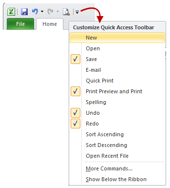

Select from the basic commands list, or click More Commands to view all options.